I’m a passionate runner. And like many data enthusiasts, I can’t resist collecting data about the things I care about. This post is both a personal reflection on my training and a hands-on tour of how Oracle can model very different questions – from streets you run most often, to the ‘feel’ of a run, to the network of your routes.
There are six very different ways to think about your running data – and each one reveals something the others cannot. I selected several runs and loaded them into a database: half marathons, interval training, long-distance running, and easy runs. The same set of GPS runs backs six completely different workloads – each asking a question the others cannot answer:
- H3 spatial heatmaps that reveal my habitual routes
- Graph queries that expose hub locations in my running network
- Time‑series gap‑filling that reconstructs missing telemetry
- Vector similarity that finds physiologically similar runs
- JSON‑relational duality views that serve your runs as API‑ready documents
- Domain‑based integrity that filters out impossible sensor readings
Each section includes simplified SQL snippets and interactive examples you can try hands-on via freesql.com. Please note that for code snippets containing a create table/view, you need to be logged into freesql.com. The full source code is available in my GitHub repository.
The Dataset
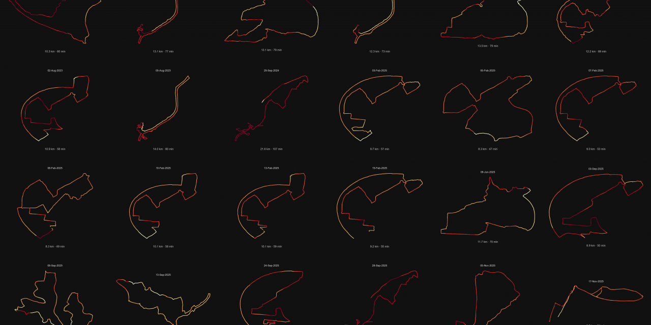
The following diagram shows some of my routes with a shape of latitude and longitude. Heart rate is colored from yellow to red depending from intensity.

The Schema
Loading starts with an Oracle External Table that reads CSV files directly. I downloaded fit-files from strava.com and converted them into CSV format. The data contains measurements with timestamp, latitude, longitude, heart rate, etc.
CREATE OR REPLACE DIRECTORY strava_dir AS '/opt/oracle/data';

CREATE TABLE strava_ext (
   ts VARCHAR2(30),
   latitude NUMBER,
   longitude NUMBER,
   altitude NUMBER,
   heart_rate NUMBER,
   ...
)
ORGANIZATION EXTERNAL (
TYPE ORACLE_LOADER
DEFAULT DIRECTORY strava_dir
ACCESS PARAMETERS (
   RECORDS DELIMITED BY NEWLINE
   SKIP 1
   FIELDS TERMINATED BY ','
)
LOCATION ('*.csv')
);
A setup script (00_setup.sql) then derives two normalised tables from the external table:
- runs: one row per activity (sport, timestamps, distance, heart-rate statistics)
- samples: one row per GPS point, foreign-keyed to its run
These two tables are the foundation every section builds on. Let’s start asking questions.
WHERE DO MY FEET ACTUALLY GO?
Spatial Heatmaps with H3
After months of running the same neighbourhood, certain streets start to feel like old friends. But memory is selective. I was convinced I explored widely – different directions, different loops. Then I looked at the data. The heatmap below tells a more honest story: I am a creature of habit. A handful of corridors dominate, run after run, regardless of what I thought I was doing.
The map reveals not just where I run, but where my routes converge – shared arteries that appear whether I’m doing an easy 7 km or pushing a long-distance effort.

Try It
Each GPS point gets assigned to a hexagonal cell. The query counts how often each cell appears and across how many distinct runs – two numbers that together reveal the shape of a training habit. High visit count, one run: obsessive repetition. High in both: a true convergence point shared across many workouts.
Tech: Spatial Indexing with H3
Raw coordinates don’t aggregate cleanly – two GPS readings one metre apart have different floating-point values and will never match in a GROUP BY. Uber’s H3 system solves this by projecting Earth onto a discrete grid of equal-area hexagons. Each point maps deterministically to one cell via Oracle’s SDO_UTIL.H3_KEY(latitude, longitude, resolution). At resolution 11 (~25 m edge length), cells are fine enough to distinguish individual lanes on a road. Once every sample carries a cell key, standard SQL aggregation does the rest – no spatial join, no geometry type, just a string GROUP BY.
WHICH JUNCTIONS HOLD MY ROUTES TOGETHER?
Graph Traversal with SQL/PGQ
After seeing the map, a new question emerged. I saw clusters of movement, but I didn’t see the connections between them. My heart rate might spike at the same location every week, but does the route take me through the same bottleneck? By treating my neighborhood as a network of nodes and edges, I could stop asking ‘Where?’ and start asking ‘How?’. This shift reveals the hidden intersections that define the flow of a city.
The map below answers that. Node size reflects how often I visited a location. Edge thickness reflects how frequently I transitioned between two locations. The brightest nodes are the real hubs – places I leave in many different directions across many different runs.

Try It
Each GPS sample maps to a ~200 m grid cell. After filtering out consecutive seconds in the same cell, transitions between cells build a directed network. The query ranks cells by out-degree – the count of distinct directions I leave from each one. Higher out-degree means a genuine junction, not just a frequently visited spot.
Tech: Property Graphs and SQL/PGQ
A relational table stores where I was. A property graph stores how I moved between places – nodes are locations, edges are transitions, and the structure itself becomes queryable. In Oracle 26ai, CREATE PROPERTY GRAPH defines a graph view directly over existing relational tables with no data migration and no separate engine.
Out-degree in pure SQL requires a self-join on an edges table. Oracle’s SQL/PGQ MATCH syntax expresses the same question as a single aggregation over a one-hop pattern (a)-[e]->(b). More complex questions (which cells connect otherwise-separate parts of the network, or which sequences of cells recur across different runs) would require chains of self-joins that grow with path length. In MATCH, the same paths appear as quantified patterns like -[IS moves_to]->{2,4}. The movement data isn’t data about a network. It is a network.
WHAT HAPPENED IN THOSE MISSING SECONDS?
Time-Series Gap-Fill
My Wednesday morning 7 km felt smooth. The watch recorded the whole thing – or so I thought. When I looked closely, four seconds were simply absent. No error message, no flag. The timestamps just jumped. For a training log that’s harmless. But the moment you want to analyse pace curves or heart-rate trends, a silent gap corrupts every calculation that crosses it.
The chart below makes those gaps visible – marked in red against the speed signal – and shows what the reconstructed trace looks like once they are filled.

Try It
The query builds a complete second-by-second reference spine, then left-joins the raw samples against it. Unmatched seconds surface as NULL and are labelled GAP. A second pass fills each gap with the average of its nearest non-null neighbours on either side.
Tech: Time-Series Reconstruction with Window Functions
Oracle’s analytic functions like LAG operate across ordered partitions without collapsing rows into aggregates. Once the spine is in place, neighbour interpolation is a single pass.
The fill strategy is a modelling decision, not a technical default. Nearest-neighbour average suits heart rate, which changes slowly and continuously. It would be wrong for cumulative distance, which must be monotonically increasing. Gap-fill encodes an assumption about how the missing value would have behaved – that assumption should be explicit and deliberate, not inherited from whichever function is convenient.
WHICH RUN FELT LIKE THE HALF-MARATHON?
Vector Similarity Search
Every runner has that feeling – the ‘Flow State’ where the body moves automatically and time compresses. My goal was to quantify this. Which training run felt exactly like my half-marathon record? Did I push myself harder in October, or was the race day effort unique? Instead of comparing distances or splits, we can compare the shape of the curve itself.
The answer surprised me: the 3×2 km interval session ranked closer to the half-marathon than the 2024 half-marathon did. And the 2024 edition showed a clearly better fitness profile than 2025. My gut would have said the opposite on both counts. The heatmap below shows pairwise similarity across all runs: the redder the cell, the more physiologically distant the pair.

Try It
Each run is represented as an 11-dimensional vector: percentage of time in each of five heart-rate zones, normalised average speed, normalised average heart rate, pace variability, and percentage of time in three pace zones. Oracle’s VECTOR_DISTANCE(v1, v2, COSINE) computes pairwise similarity in a single function call.
| Dimensions | Meaning |
|---|---|
| 1–5 | % time in HR zones 1–5 |
| 6 | Normalised average speed |
| 7 | Normalised average HR |
| 8 | Speed coefficient of variation |
| 9–11 | % time in pace zones slow / moderate / fast |
Tech: Vector Search and Cosine Distance
A vector embedding maps an object to a point in high-dimensional space such that similar objects land close together. Here the embedding is hand-crafted from domain knowledge: heart-rate zone distributions are a well-understood physiological proxy for effort type. For text, images, or audio, an embedding model – a neural network – produces the vector automatically.
Cosine distance measures the angle between two vectors, not their length. It is appropriate when magnitude is irrelevant and only direction matters: two runs with the same intensity distribution but different durations should match, and they do. Oracle’s VECTOR datatype stores fixed-dimension float arrays natively, and vector indexes (HNSW, IVF) make similarity search fast at scale without scanning every row. If you want to read more about vectors and their visualization, see my article Spotify music clustering with Oracle AI Vector: From vectors to visual insights.
HOW WOULD A PHONE APP RETRIEVE A RUN?
JSON-Relational Duality Views
A training app doesn’t think in tables. It expects a single JSON document per run – metadata at the top, GPS samples nested below – ready to render on screen. The database, meanwhile, stores runs and samples in two separate normalised tables, because that is the right way to store them. Historically, serving both meant either duplicating data or writing transformation logic in application code.
The response below is what the app receives: one JSON object, run metadata at the top, GPS samples embedded as an array. The database assembled it from the same normalised rows used by every other query in this article.
The response is a single JSON object like:
{
  "_id": 5,
  "filename": "HM_Ulm_2025.csv",
  "sport": "running",
  "distance": 21.3,
  "samples": [
    {
      "sampleId": 40001,
      "ts": "2025-09-28T07:23:28.000Z",
      "lat": 48.3981, "lon": 9.9924,
      "altitude": 476, "speed": 0.0, "heartRate": 87
    },
    {
      "sampleId": 40002,
      "ts": "2025-09-28T07:23:29.000Z",
      "lat": 48.3981, "lon": 9.9925,
      "altitude": 476, "speed": 0.5, "heartRate": 88
    },
    "..."
  ]
}
Try It
A duality view is defined once over the existing runs and samples tables. The app queries it like a document store: SELECT data FROM run_dv WHERE ... and gets a fully nested JSON object back. Writes through the view update the underlying relational tables directly, maintaining all constraints and indexes.
The true power here is the transparency. The database does not care if I treat this data as rows in a table for reporting, or documents for an API call. I can switch between these mental models instantly. This eliminates the friction of ETL processes – I no longer need to transform my data just to serve it differently.
Tech: JSON-Relational Duality
Oracle’s duality views allow a relational schema and a document schema to coexist over the same data without copying it. The view definition specifies which columns become JSON fields and how child rows are nested as arrays. The database handles assembly and disassembly transparently.
This eliminates the classic tension between normalisation and API convenience. The relational model is preserved for analytics with joins, aggregations, constraints, while the document model is preserved for application integration. Neither side compromises, and there is no ETL between them.
WHAT DOES THE DATABASE SIMPLY REFUSE TO STORE?
Domain-Based Integrity
GPS watches produce messy telemetry. A sensor glitch might log a heart rate of 999 bpm. A coordinate conversion error might produce a latitude of 200 degrees. Both are syntactically valid numbers. Both are physically impossible. And in a system without explicit constraints, both will land silently in the database and corrupt every downstream calculation that touches them.
I wanted the database itself to be the gatekeeper, not a validation script run occasionally, not a note in the documentation, but a rule encoded in the schema that makes invalid data impossible to store in the first place.
Try It
Three domains encode the physical limits of each measurement: latitude between −90 and 90, longitude between −180 and 180, speed greater than or equal to zero. A samples_typed view applies these domains across the full dataset. An attempt to insert a value outside any domain fails at write time with a constraint violation before the bad data reaches a single table. So you will see an error message when executing the code. You can correct it as described at the end of the code block.
Tech: Relational Domains and Constraint Enforcement
A domain in SQL is a named data type with attached constraints: a reusable specification of what values are physically valid for a given measurement. CREATE DOMAIN ... defines the rule once; every column declared with that domain inherits it automatically.
Constraints defined in the schema are self-documenting, always enforced, and visible to every tool that inspects the schema. Constraints defined in application code are enforced only when that code runs, in the version that was deployed, by the developer who remembered to call it. The schema is the single source of truth for what the data is allowed to be.
Conclusion
I started this project because I enjoy running and I enjoy data. I wanted to analyze my runs while experimenting with the latest Oracle version. I ended with several workloads within the same multi-model database:
- Spatial indexing
- Time-series reconstruction
- Vector similarity
- Graph traversal
- JSON document assembly
- Relational integrity
Every query in this article runs against Oracle 26ai. Rather than stitching together separate engines for spatial, graphs, vector, timeseries, JSON and relational, Oracle 26ai lets all of these patterns live in a single multi‑model / converged database. If you are interested in Formula 1 data, I created similiar scenarios in my article One Database, Six Workloads: Analyzing F1 Telemetry With Oracle Converged Database.
While experimenting with Oracle and writing this article, I learned a lot about its new multi‑model features. At the same time, I uncovered some surprisingly concrete insights about my running – for example, the vector search showed clearly that the half‑marathon from 2024 had a better fitness profile than my half‑marathon in 2025 and a surprisingly similar profile to a shorter interval session. That alignment actually makes perfect sense when I look at the data, even though my gut feeling would have suggested the two half‑marathons are closer to each other!