CREATE TABLE IF NOT EXISTS test_embedding (
     id SERIAL PRIMARY KEY
   , embedding vector
   , created_at timestamptz DEFAULT now()
);

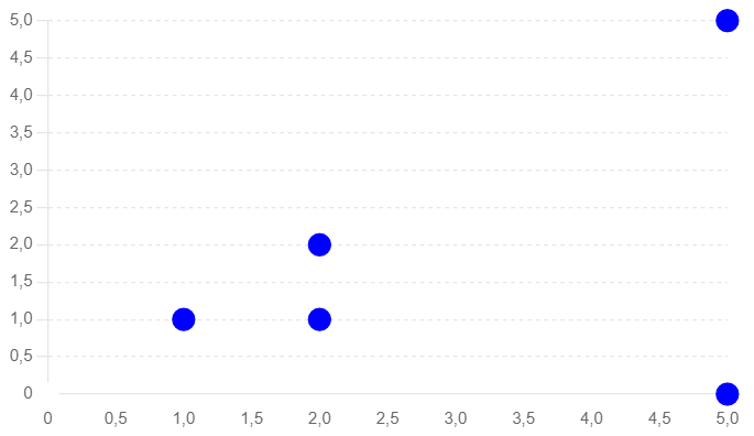
INSERT INTO test_embedding (embedding) VALUES (ARRAY[1, 1]);
INSERT INTO test_embedding (embedding) VALUES (ARRAY[2, 2]);
INSERT INTO test_embedding (embedding) VALUES (ARRAY[2, 1]);
INSERT INTO test_embedding (embedding) VALUES (ARRAY[5, 5]);
INSERT INTO test_embedding (embedding) VALUES (ARRAY[5, 0]);- Euclidean Distance (L2)
- Cosine Similarity
- Manhattan Distance
- Dot Product (L1)
- Hamming Distance
- Jaccard Similarity
Similarity search algorithms
The following paragraphs explain the different algorithms with an SQL example for PostgreSQL pg_vector extension. The SQL statements compare each vector with one another using a Cartesian cross join (intentionally).
For Euclidian Distance, Cosine Similarity, Manhattan Distance, and Dot Product exist operators in pg_vector. For the two other algorithms (Hamming Distance and Jaccard Similarity) stored procedures have been created. The stored procedures just show the principle and are not tuned for speed (for usage in production systems).
At the end of the article, the algorithms are compared.
Search algorithm: Euclidean Distance (L2)
Euclidean distance measures how far two points are from each other in a straight line. It’s like using a ruler to measure the distance between two dots on a paper.
Mathematical Formula: d(p, q) = sqrt((q1 – p1)^2 + (q2 – p2)^2 + … + (qn – pn)^2)
SELECT a.id, b.id
     , a.embedding as embedding_a
     , b.embedding as embedding_b
     , round((a.embedding <-> b.embedding)::numeric, 5) AS l2_euclidean_distance
FROM test_embedding a
   , test_embedding b
ORDER BY a.embedding, b.embedding;
Search algorithm: Cosine Similarity
Cosine similarity measures how similar two items are, regardless of their size. Imagine comparing the angle between two arrows pointing in different directions; the closer the angle is to zero, the more similar the items are.
Mathematical Formula: cosine_distance(p, q) = 1 – ( (p1*q1 + p2*q2 + … + pn*qn) / (sqrt(p1^2 + p2^2 + … + pn^2) * sqrt(q1^2 + q2^2 + … + qn^2)) )
Cosine Distance is also used with formula cosine_distance(p, q) = 1 – cosine_similarity(p, q).
SELECT a.id, b.id
     , a.embedding as embedding_a
     , b.embedding as embedding_b
     , round((a.embedding <=> b.embedding)::numeric, 5) AS cosine_similarity
FROM test_embedding a
   , test_embedding b
ORDER BY a.embedding, b.embedding;
Search algorithm: Manhattan Distance
Manhattan distance measures the total distance traveled between two points if you can only move along grid lines (like streets in a city). It’s like walking in a city where you can only move north-south or east-west.
Mathematical Formula: manhattan_distance(p, q) = |q1 – p1| + |q2 – p2| + … + |qn – pn|
SELECT a.id, b.id
     , a.embedding as embedding_a
     , b.embedding as embedding_b
     , round((a.embedding <+> b.embedding)::numeric, 5) AS l1_manhattan_distance
FROM test_embedding a
   , test_embedding b
ORDER BY a.embedding, b.embedding;
Search algorithm: Dot Product (L1)
The dot product measures how much two vectors point in the same direction. Imagine you have two arrows; the dot product tells you how much they overlap if they were placed on top of each other.
Mathematical Formula: dot_product(p, q) = p1*q1 + p2*q2 + … + pn*qn
SELECT a.id, b.id
     , a.embedding as embedding_a
     , b.embedding as embedding_b
     , - round((a.embedding <#> b.embedding)::numeric, 5) AS dot_product
FROM test_embedding a
     , test_embedding b
ORDER BY a.embedding, b.embedding;
Search algorithm: Hamming Distance
Hamming distance measures how many places two strings of equal length differ. It’s like comparing two words to see how many letters are different.
Mathematical Formula: hamming_distance(p, q) = count(p_i != q_i for i from 1 to n)
(Here, count(p_i != q_i for i from 1 to n) counts the number of positions where the corresponding elements of p and q are different.)
CREATE OR REPLACE FUNCTION hamming_distance(vec1 vector, vec2 vector)
RETURNS int AS $$
DECLARE
    distance int := 0;
    i int;
    vec1_elements float8[];
    vec2_elements float8[];
BEGIN
    -- Convert vectors to arrays
    vec1_elements := regexp_split_to_array(trim(both '[]' from vec1::text), ',')::float8[];
    vec2_elements := regexp_split_to_array(trim(both '[]' from vec2::text), ',')::float8[];

    -- Ensure the vectors are of the same dimension
    IF array_length(vec1_elements, 1) != array_length(vec2_elements, 1) THEN
        RAISE EXCEPTION 'Vectors must have the same number of dimensions';
    END IF;

    -- Calculate the Hamming distance
    FOR i IN 1..array_length(vec1_elements, 1) LOOP
        IF vec1_elements[i] != vec2_elements[i] THEN
            distance := distance + 1;
        END IF;
    END LOOP;

    RETURN distance;
END;
$$ LANGUAGE plpgsql IMMUTABLE;

SELECT a.id, b.id,
     , a.embedding AS embedding_a
     , b.embedding AS embedding_b
     , hamming_distance(a.embedding, b.embedding) AS hamming_distance
FROM test_embedding a
   , test_embedding b
ORDER BY a.embedding, b.embedding;
Search algorithm: Jaccard Similarity
Jaccard similarity measures how similar two sets are by comparing their common elements. It’s like comparing two groups of friends and seeing how many friends they have in common.
Mathematical Formula: jaccard_similarity(A, B) = |A ∩ B| / |A ∪ B|
(Here, A and B are sets, |A ∩ B| is the number of elements in the intersection of A and B, and |A ∪ B| is the number of elements in the union of A and B.)
Jaccard Distance is also used with the formula jaccard_distance(A, B) = 1 – (|A ∩ B| / |A ∪ B|)
CREATE OR REPLACE FUNCTION jaccard_similarity(vec1 vector, vec2 vector)
RETURNS numeric AS $$
DECLARE
    intersection_count int := 0;
    union_count int := 0;
    i int;
    vec1_elements float8[];
    vec2_elements float8[];
BEGIN
    -- Convert vectors to arrays
    vec1_elements := regexp_split_to_array(trim(both '[]' from vec1::text), ',')::float8[];
    vec2_elements := regexp_split_to_array(trim(both '[]' from vec2::text), ',')::float8[];

    -- Ensure the vectors are of the same dimension
    IF array_length(vec1_elements, 1) != array_length(vec2_elements, 1) THEN
        RAISE EXCEPTION 'Vectors must have the same number of dimensions';
    END IF;

    -- Calculate the intersection and union
    FOR i IN 1..array_length(vec1_elements, 1) LOOP
        IF vec1_elements[i] = 1 AND vec2_elements[i] = 1 THEN
            intersection_count := intersection_count + 1;
        END IF;
        IF vec1_elements[i] = 1 OR vec2_elements[i] = 1 THEN
            union_count := union_count + 1;
        END IF;
    END LOOP;

    IF union_count = 0 THEN
        RETURN 0;
    END IF;

    RETURN (intersection_count::numeric / union_count::numeric);
END;
$$ LANGUAGE plpgsql IMMUTABLE;


SELECT a.id, b.id
     , a.embedding AS embedding_a
     , b.embedding AS embedding_b
     , round(jaccard_similarity(a.embedding, b.embedding), 5) AS jaccard_similarity
FROM test_embedding a
   , test_embedding b
ORDER BY a.embedding, b.embedding;
Results of similarity searches with PostgreSQL
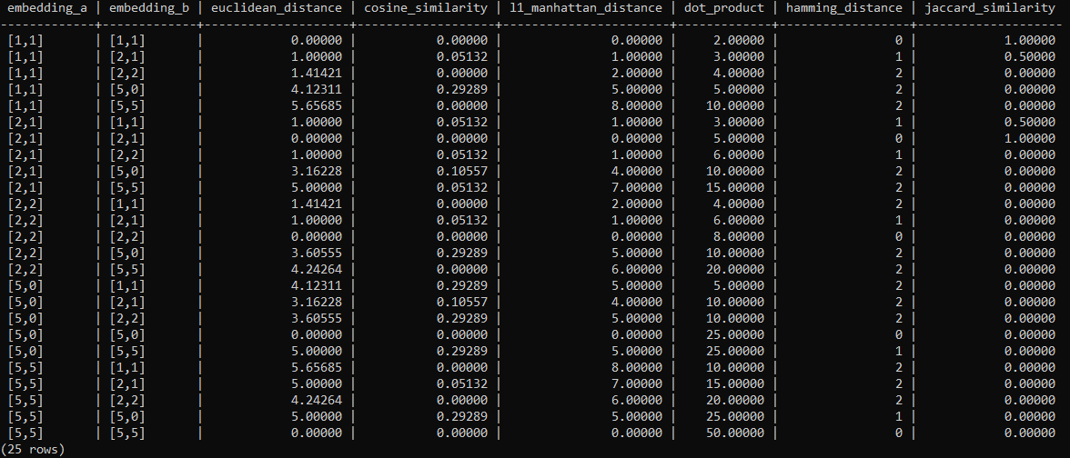
The following table lists the results using the algorithms explained above. All results were computed by using pg_vector and the SQL statements from the article.
The following SQL statement creates one table containing 25 rows (5×5 as each vector is compared with one another ) and all algorithms.
SELECT a.id AS id_a, b.id AS id_b
     , a.embedding AS embedding_a
     , b.embedding AS embedding_b
     , round((a.embedding <-> b.embedding)::NUMERIC, 5) AS euclidean_distance
     , round((a.embedding <=> b.embedding)::NUMERIC, 5) AS cosine_similarity
     , round((a.embedding <+> b.embedding)::numeric, 5) AS l1_manhattan_distance
     , - round((a.embedding <#> b.embedding)::numeric, 5) AS dot_product
     , hamming_distance(a.embedding, b.embedding) AS hamming_distance
     , round(jaccard_similarity(a.embedding, b.embedding), 5) AS jaccard_similarity
FROM test_embedding a
   , test_embedding b;

Comparison of search algorithms in vector databases
The following table lists strengths, weaknesses, and recommendations for the above explained algorithms.
| Strengths | Weaknesses | Recommendations | |
| Euclidian Distance |
|
|
Use Euclidean distance when working with low-dimensional data or when simplicity and ease of understanding are important. Ensure data is normalized. |
| Cosine Similarity |
|
|
Use cosine similarity for text data, document comparison, and other high-dimensional data where scale invariance is important. Normalization is optional, but common. |
| Manhattan Distance |
|
|
Use Manhattan distance for grid-based systems, pathfinding in grid-like structures, and when simplicity and ease of understanding are important. Ensure data is normalized. |
| Dot Product |
|
|
Use the dot product for comparing the direction of vectors, especially when magnitude is relevant, such as in certain machine learning and data analysis tasks. |
| Hamming Distance |
|
|
Use Hamming distance for error detection and correction in binary strings or comparing fixed-length data. |
| Jaccard Similarity |
|
|
Use Jaccard similarity for comparing sets, binary data, or categorical attributes where common elements are significant. |
Note that some algorithms require normalization of the data. Normalization means scaling the data so that it falls within a specific range, usually between 0 and 1. This is particularly important when different features of the data have different units or magnitudes. Normalization helps eliminate the influence of varying scales and ensures that all features are treated equally.
When vectors are normalized, the dot product of the normalized vectors is equivalent to the cosine similarity of the original vectors
A common method for normalization is min-max scaling, where the values of a feature are scaled to a range between 0 and 1:
normalized_value = (value – min_value) / (max_value – min_value)
Another method is z-score normalization, where the values are scaled based on their mean and standard deviation:
normalized_value = (value – mean) / standard_deviation
Summary
Similarity search in vector databases is a powerful tool that enables finding items that are semantically similar rather than exactly the same. Each algorithm has its strengths and weaknesses, and knowing when to use each one will help you make the most of your similarity search applications.
Perfomance may suffer if the algorithms are used for huge datasets. Vector Indexes will help to improve performance but penalties in accuracy might be the trade-off.

