Vector indexes are crucial for semantic search performance, optimizing efficient querying. In this article, I will delve into various types of vector indexes, their workings, pros and cons, and recommendations for their use. The article also provides a practical example using PostgreSQL’s pgvector extension, demonstrating the use of indexes such as IVF and HNSW, including the difference between exact and approximate nearest neighbor (aKNN) searches.
Optimizing Performance in Vector Searches
Optimizing performance in vector searches can be achieved through two primary strategies:
- Reducing the Search Scope: This involves using indexes for restricting the search to the nearest clusters, which minimizes the number of comparisons needed.
- Reducing Vector Size: This strategy reduces the number of bits used to represent vector values, leading to faster computations and lower memory usage. This optimization strategy is not part of this article.
Types of Vector Indexes
There exist a variety of vector indexes. The article fcosuses on the two main indexes
- Inverted File (IVF)
- Hierarchical Navigable Small World (HNSW)
Inverted File (IVF)
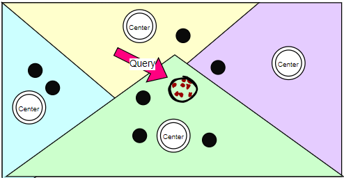
Idea and How It Works: The Inverted File (IVF) index partitions the data space into a finite number of cells using a clustering algorithm (e.g., k-means). Each cell contains a list of vectors that fall within its boundaries. When querying, the nearest partition(s) are examined to find the closest vectors to the query vector.
The picture shows that if the green partition is chosen, only vectors within the partition is considered even if there are closer vectors in other partitions (approximate search). It can be configured how many partitions are used for querying.
Pros:
- Efficient for large-scale datasets.
- Good balance between search speed and accuracy.
- Scalable.
Cons:
- Index construction can be computationally expensive.
- Requires tuning of parameters like the number of partitions.
Recommendation: Use IVF when you have a large dataset and need a balanced solution between search speed and accuracy. It’s particularly useful for scenarios where the dataset is static or changes infrequently.
Hierarchical Navigable Small World (HNSW)
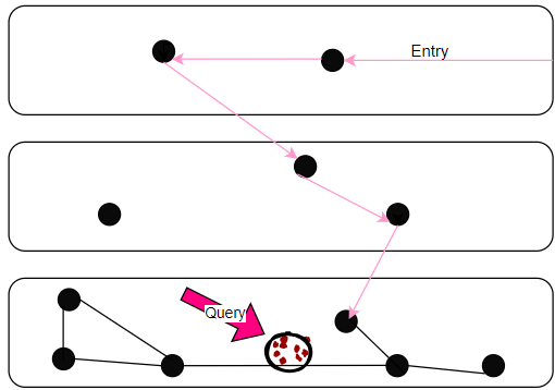
Idea and How It Works: HNSW is a graph-based index that organizes data points into a multi-layered graph. Each layer is a small-world network, allowing fast navigation between vectors. Queries traverse this graph to find the nearest neighbors, starting from a randomly selected node (entry node in the picture) and moving through the layers closer to the target vector. If there is no neighbor closer to the query than the current node, the local minimum is found and returned.
Pros:
- Very fast query times.
- Often high accuracy.
Cons:
- High memory usage (therefore not suited for very huge datasets)
- Index construction can be slow.
Recommendation: HNSW is ideal for applications requiring real-time search with high accuracy, such as recommendation systems and personalized search. Its performance is particularly advantageous for dynamic datasets with frequent updates.
Example with PostgreSQL pg_vector
Now let’s have a look how to create IVF and HNSW indexes using PostgreSQL and performing exact and approximate searches. For an introduction into vector databases and embeddings see my article Vector databases: what, why, and how. The article also shows how to set up pg_vector extension in PostgreSQL.
First create a table for storing vector data and populating the table with 4 defined rows and 10.000 randomly created data. With a few rows only, an index would not be used by the database optimizer.
CREATE TABLE items (
    id serial PRIMARY KEY
  , embedding vector(3)
);

INSERT INTO items (embedding)
VALUES
    ('[0.1, 0.2, 0.3]'),
    ('[0.2, 0.3, 0.4]'),
    ('[0.3, 0.4, 0.5]'),
    ('[0.4, 0.5, 0.6]');

-- Generate 10,000 rows with random data in the specified range
INSERT INTO items (embedding)
SELECT ARRAY[
    0.6 + (random() * (0.3)),
    0.7 + (random() * (0.2)),
    0.8 + (random() * (0.1))
]::vector(3)
FROM generate_series(1, 10000);
The following commands show how to create IVF and HSNW indexes.
CREATE INDEX items_ivf ON items USING ivfflat (embedding) WITH (lists = 10);
DROP INDEX items_ivf;

CREATE INDEX items_hnsw ON items
USING hnsw (embedding vector_l2_ops) WITH (m = 16, ef_construction = 200);
DROP INDEX items_hnsw;
The query retrieves the top 3 similarity vectors.
SELECT id, embedding
FROM items
ORDER BY embedding <-> '[0.15, 0.25, 0.35]'
LIMIT 3;
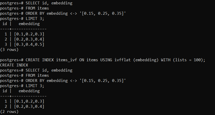
The first example runs the query on the table without an index (exact search), then creates the IVF index with 100 lists and reruns the query. The index returns two rows only compared to the exact search. Obviously the clustering into lists is not optimal.
The exact search without an index compares every entry in the table with the data in the where clause. Indexes support an approximate search where some data is skipped depending how the index is created.
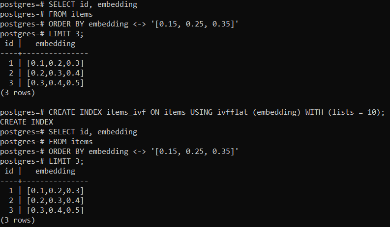
The second example runs the query on the table without an index (exact search), then creates the IVF index with 10 lists and reruns the query. The index now returns also three rows.
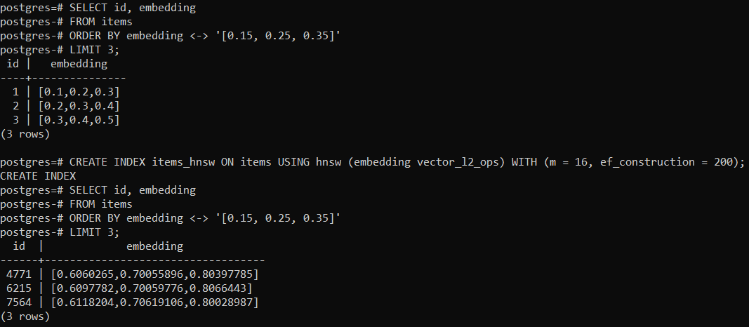
The third example runs the query on the table without an index (exact search), then creates the HNSW index and reruns the query. The index returns different rows though.
Conclusion
Choosing the right vector index depends on your specific use case, data characteristics, and performance requirements. IVF and HNSW are popular choices. The example shows that indexes will often lead to approximate searches instead of exact results. Balance between speed and accuracy must be considered when configuring indexes.


