One Database, Six Workloads: Analyzing F1 Telemetry With Oracle Converged Database

The Complexity We Created

Somewhere along the way, we convinced ourselves that specialized databases were the answer to everything. Need to store documents? Spin up DocumentDB X1. Time series data? Here’s TimeseriesDB X2. Graph relationships? GraphDB X3. Vector embeddings for AI? VectorDB X4. Spatial queries? SpatialDB X5. And finally use relationalDB X6 to store structured data,

Before you know it, your “modern data architecture” looks like a technology zoo: six databases, six connection pools, six backup strategies, six security models, and one exhausted operations team trying to keep it all running.

This is polyglot persistence—the idea that each data problem deserves its own specialized database. It sounds elegant in architecture diagrams. In production, it’s a maintenance nightmare.

What if there was a simpler way?

The Converged Alternative

Oracle calls it the “Converged Database” or a multi-modal database in general terms – a single database engine that natively supports multiple data models and workloads. Not through awkward adapters or bolted-on extensions, but as first-class citizens with dedicated syntax, optimized storage, and proper indexing.

One database. One backup. One security model. One query language that works across all your data.

This isn’t about Oracle being a jack of all trades and master of none. It’s about recognizing that most enterprise data problems aren’t isolated – they’re interconnected. Your relational facts reference your JSON documents. Your time series correlates with your spatial coordinates. Your graph relationships emerge from your dimensional model.

When all your data lives in one place, these connections become queries instead of ETL pipelines.

Let me show you what this looks like in practice.

The Demo: Formula 1 Race Analytics

To demonstrate multi-modal capabilities, I built a complete data pipeline using real Formula 1 telemetry data. The 2024 Singapore Grand Prix serves as our dataset—62 laps of racing, 20 drivers, nearly a million telemetry samples, and dozens of race control messages.

The full code is available at: https://github.com/abuckenhofer/fastf1-oracleconverged

The README covers installation and setup. Here, I want to focus on the why, how, and what of each capability.

Relational: The Foundation That Still Matters

Why

Despite the NoSQL revolution, relational modeling remains unmatched for representing business entities and their relationships. Drivers belong to teams. Teams compete in events. Results connect drivers to finishing positions. It’s been working for decades because it mirrors how businesses actually think about their data.

How

Oracle’s relational engine lays the foundation with robust constraints and ACID compliance. But it creates a true hybrid engine using the In-Memory Columnar option. By transparently maintaining large fact tables in a compressed columnar format in RAM, the database executes transactional and analytical workloads simultaneously without conflict.

What

Consider this question: How does tire degradation affect lap times throughout a stint?

SELECT
   d.driver_code,
   l.stint_number,
   l.lap_number,
   l.tyre_life,
   ROUND(l.lap_time_sec, 3) AS lap_time,
   ROUND(l.lap_time_sec - LAG(l.lap_time_sec) OVER (
   PARTITION BY l.driver_id, l.stint_number
      ORDER BY l.lap_number
      ), 3) AS delta_to_previous,
   ROUND(l.lap_time_sec - FIRST_VALUE(l.lap_time_sec) OVER (
      PARTITION BY l.driver_id, l.stint_number
      ORDER BY l.lap_number
      ), 3) AS degradation_from_stint_start
FROM fact_lap l
JOIN dim_driver d ON l.driver_id = d.driver_id
WHERE l.is_accurate = 1
ORDER BY d.driver_code, l.stint_number, l.lap_number;

The LAG function compares each lap to the previous one. FIRST_VALUE anchors the comparison to the stint’s opening lap. No temporary tables. No procedural code. Just declarative SQL expressing exactly what we want to know.

Or consider driver consistency—who delivers the most predictable lap times?

SELECT
   d.driver_code,
   d.full_name,
   COUNT(*) AS valid_laps,
   ROUND(AVG(l.lap_time_sec), 3) AS avg_lap_time,
   ROUND(STDDEV(l.lap_time_sec), 4) AS consistency,
   RANK() OVER (ORDER BY STDDEV(l.lap_time_sec)) AS consistency_rank
FROM fact_lap l
JOIN dim_driver d ON l.driver_id = d.driver_id
WHERE l.is_accurate = 1 AND l.lap_time_sec < 120
GROUP BY d.driver_id, d.driver_code, d.full_name
ORDER BY consistency_rank;

Fernando Alonso emerges as the most consistent driver in Singapore – his standard deviation of just 0.6 seconds across 58 laps speaks to the precision of his racecraft. That can be seen in the following image: driver consistency comparison – box plots showing lap time distributions for each driver, sorted by standard deviation (most consistent first). The narrow boxes indicate repeatable performance; wider boxes show erratic pace. This visualization showcases STDDEV and PERCENTILE_CONT to quantify driving precision.

JSON: Flexibility Without Abandoning Structure

Why

Not all data arrives in neat rows and columns. Race control messages have variable fields. Session metadata contains nested structures. External APIs return JSON. You need a place to land this data without forcing it into a rigid schema – but you also need to query it alongside your relational data.

How

Oracle stores JSON in a native format. The magic happens with JSON_VALUE for scalar extraction and JSON_TABLE for transforming documents into relational result sets. Your JSON becomes queryable with standard SQL.

What

Race control messages arrive as semi-structured data—flags, incidents, penalties, DRS status changes. Each message type has different fields.

SELECT
   JSON_VALUE(d.payload, '$.Category') AS category,
   JSON_VALUE(d.payload, '$.Flag') AS flag,
   JSON_VALUE(d.payload, '$.Message') AS message_text,
   JSON_VALUE(d.payload, '$.Lap' RETURNING NUMBER) AS lap
FROM f1_raw_documents d
WHERE d.doc_type = 'race_control_message'
ORDER BY d.doc_id;

The session metadata contains deeply nested information about the circuit, country, and official event name:

SELECT
   JSON_VALUE(payload, '$.session_id') AS session_id,
   JSON_VALUE(payload, '$.data.Meeting.OfficialName') AS official_name,
   JSON_VALUE(payload, '$.data.Meeting.Location') AS location,
   JSON_VALUE(payload, '$.data.Meeting.Country.Name') AS country
FROM f1_raw_documents
WHERE doc_type = 'session_info';

No separate document database. No data duplication. The JSON lives alongside the relational data and joins seamlessly with dimension tables.

The following image shows the JSON document structure – a treemap visualization of the session_info document, visualizing the nested hierarchy of F1 session metadata. Each rectangle represents a JSON key, with size indicating the depth of nesting. This semi-structured data coexists with relational tables and can be queried with standard SQL using JSON_VALUE and JSON_TABLE.

Time Series: When Every Millisecond Counts

Why

Modern F1 cars generate gigabytes of telemetry per race. Speed, RPM, throttle position, brake pressure, gear selection—all sampled hundreds of times per second. This is time series data: high-volume, append-mostly, and queried primarily by time ranges. Traditional row-by-row relational storage struggles with this volume.

How

Oracle handles time series through optimized indexing on timestamp columns, efficient bulk loading and the possibility to query tables in a compressed columnar format in RAM. While specialized time series databases exist, Oracle’s strength is correlation – joining telemetry with lap data, driver information, and track status in a single query.

What

Where do drivers brake hardest? This query identifies heavy braking events across the entire race:

SELECT
   d.driver_code,
   COUNT(*) AS braking_events,
   ROUND(AVG(t.speed), 1) AS avg_entry_speed,
   ROUND(MAX(t.speed), 1) AS max_entry_speed
FROM fact_telemetry t
JOIN dim_driver d ON t.driver_id = d.driver_id
WHERE t.brake = 1 AND t.speed > 150
GROUP BY d.driver_id, d.driver_code
ORDER BY braking_events DESC;

Charles Leclerc recorded 588 heavy braking events – more than any other driver – with entry speeds reaching 312 km/h. This kind of analysis, correlating telemetry patterns with driver identity, requires joining across data models.

Weather correlation adds another dimension:

SELECT
   ROUND(time_sec / 60, 0) AS race_minute,
   ROUND(air_temp, 1) AS air_temp_c,
   ROUND(track_temp, 1) AS track_temp_c,
   humidity AS humidity_pct,
   rainfall
FROM fact_weather
WHERE time_sec > 3400
ORDER BY time_sec;

Singapore’s night race maintains remarkably stable conditions—track temperature varying by less than 2 degrees throughout. In a rain-affected race, this same query would reveal the conditions that triggered tire strategy changes.

Real-world time series data often has gaps—missing samples, irregular intervals, or sensor dropouts. Oracle’s MODEL clause provides powerful gap-filling capabilities directly in SQL for continuous time intervals:

WITH weather_calc AS (
   SELECT 
   event_id, 
   FLOOR(time_sec / 60) AS minute_bucket, 
   air_temp, 
   track_temp
   FROM fact_weather
)
SELECT minute_bucket, air_temp, track_temp, is_interpolated
FROM weather_calc
   MODEL
   PARTITION BY (event_id)
   DIMENSION BY (minute_bucket)
   MEASURES (air_temp, track_temp, 0 AS is_interpolated)
   RULES AUTOMATIC ORDER (
   -- Interpolate AIR_TEMP with forward-fill
      air_temp[FOR minute_bucket FROM 0 TO 120 INCREMENT 1] =
      CASE 
         WHEN air_temp[CV()] IS NULL THEN air_temp[CV()-1]
         ELSE air_temp[CV()]
      END,
   -- Flag the interpolated rows
   is_interpolated[FOR minute_bucket FROM 0 TO 120 INCREMENT 1] =
      CASE 
        WHEN air_temp[CV()] IS NULL THEN 1 
        ELSE 0 
      END
   )
ORDER BY minute_bucket;

The MODEL clause treats query results as a spreadsheet, allowing cell-by-cell calculations with references like CV()-1 (previous cell) and CV()+1 (next cell). This enables linear interpolation, forward fill, or any custom gap-filling logic – all within a single SQL statement. For telemetry data sampled at irregular intervals, this means creating continuous timelines without application-layer processing.

The following image shows the position chart – the classic F1 race progression visualization. Lines show each driver’s position throughout the race, colored by team. Crossings indicate overtakes, vertical movements show pit stop position shuffles. This uses Oracle’s LAG window function to detect position changes lap-by-lap, with an annotation highlighting the driver who gained the most positions during the race.

Spatial: Location as a First-Class Citizen

Why

F1 telemetry includes X/Y coordinates for every sample—the car’s position on the track. Spatial queries let you ask location-based questions: Which corners see the most overtakes? Where do cars run closest together? What’s the racing line through turn 7?

How

Oracle Spatial uses the SDO_GEOMETRY type with dedicated spatial indexes. Points, lines, polygons – all queryable with functions like SDO_WITHIN_DISTANCE (proximity search) and SDO_INTERSECTION (overlap detection).

What

Let’s analyze driving patterns by track sector:

SELECT
   d.driver_code,
   CASE
      WHEN ts.geom.SDO_POINT.X > 800 AND ts.geom.SDO_POINT.Y > 1000 THEN 'SECTOR_1'
      WHEN ts.geom.SDO_POINT.X < 200 AND ts.geom.SDO_POINT.Y > 500 THEN 'SECTOR_2'
      ELSE 'SECTOR_3'
   END AS track_sector,
   COUNT(*) AS samples,
   ROUND(AVG(ts.speed), 1) AS avg_speed,
   ROUND(MAX(ts.speed), 1) AS max_speed
FROM telemetry_spatial ts
JOIN dim_driver d ON ts.driver_id = d.driver_id
GROUP BY d.driver_id, d.driver_code,
   CASE
      WHEN ts.geom.SDO_POINT.X > 800 AND ts.geom.SDO_POINT.Y > 1000 THEN 'SECTOR_1'
      WHEN ts.geom.SDO_POINT.X < 200 AND ts.geom.SDO_POINT.Y > 500 THEN 'SECTOR_2'
      ELSE 'SECTOR_3'
   END
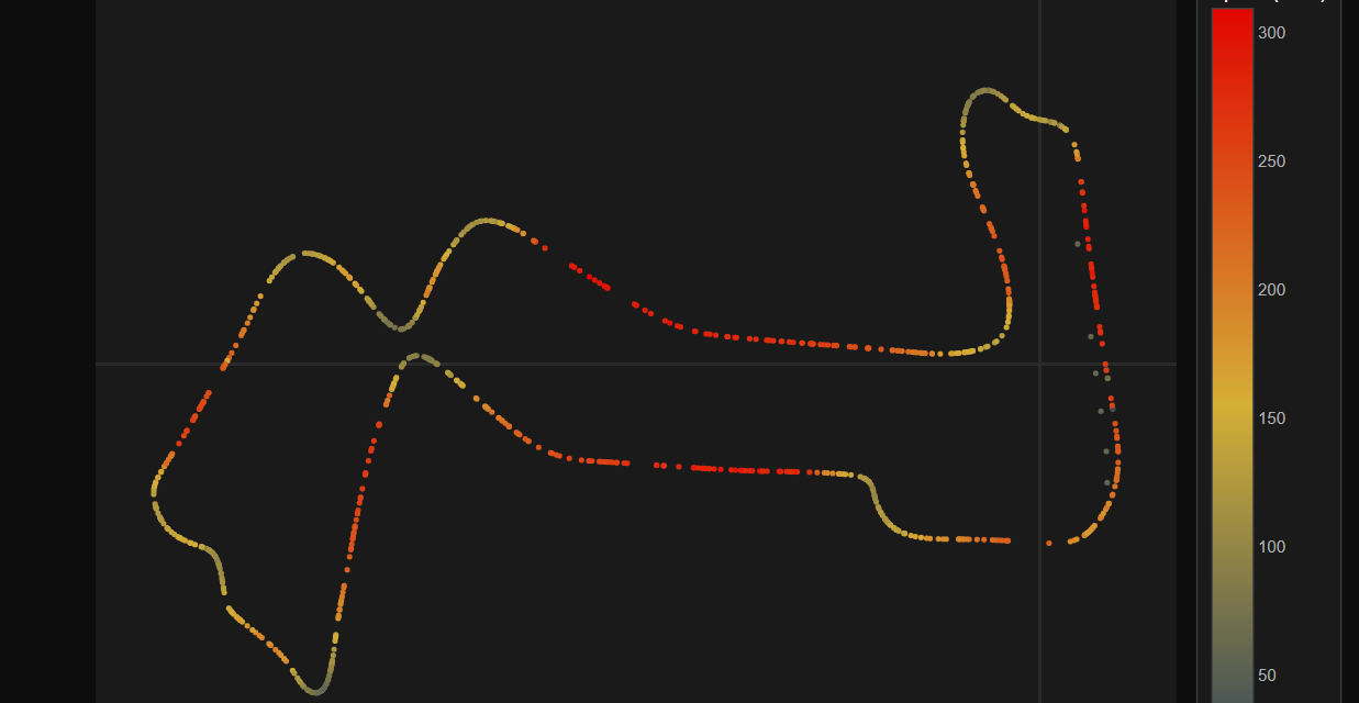
ORDER BY d.driver_code, track_sector;

The spatial coordinates, combined with speed data, reveal which drivers carry more speed through the technical sectors versus the high-speed sections.In a dedicated spatial database, you’d have the geometry but lose the connection to lap times, tire compounds, and fuel loads. In a multi-modal SQL database, it’s all one query.
The image shows Spatial telemetry on the Marina Bay Circuit – an interactive map with car positions converted from telemetry x/y coordinates to geographic latitude/longitude. Points are colored by speed (blue=slow through corners, red=fast on straights), with braking zones highlighted. This visualization demonstrates Oracle’s SDO_GEOMETRY capabilities storing real track positions that can be queried with spatial functions like SDO_WITHIN_DISTANCE.

Graph: Relationships as Data

Why

Some questions are fundamentally about connections. Who are teammates? Which drivers have raced for the same team? How many degrees of separation exist between two drivers through shared team history? These graph traversal problems are awkward in relational SQL but natural in graph query languages.

How

SQL Property Graph provides graph structures defined over existing relational tables with GRAPH_TABLE queries using pattern matching syntax. Your dimensions become vertices; your bridge tables become edges. No data duplication, no synchronization headaches.

What

Finding teammates becomes a graph pattern match:

SELECT driver1_code, team_name, driver2_code
FROM GRAPH_TABLE (f1_graph
   MATCH (d1 IS driver) -[dt1 IS drives_for]-> (t IS team)
   <-[dt2 IS drives_for]- (d2 IS driver)
WHERE d1.driver_id < d2.driver_id
   COLUMNS (
      d1.driver_code AS driver1_code,
      t.team_name AS team_name,
      d2.driver_code AS driver2_code))
ORDER BY team_name;

The pattern (driver)-[drives_for]->(team)<-[drives_for]-(driver) expresses “two drivers connected through the same team” more intuitively than the equivalent self-join. Scale this to a full season – or a decade of driver movements – and the graph model becomes indispensable.
The result could be a graph showing an overtake network – a directed graph visualization showing who overtook whom during the race. Arrows point from the overtaking driver to the overtaken driver, with line thickness indicating the number of passes. Node size reflects net positions gained or lost. This visualization uses relational lap data to detect position changes between consecutive laps, demonstrating intuitive pattern matching like “find drivers who were overtaken and later recovered the position.”

Vector: Semantic Search Meets Structured Data

Why

The rise of large language models has created a new data type: embeddings. These high-dimensional vectors capture semantic meaning, enabling similarity search that understands concepts rather than just keywords. “Find messages about dangerous driving” should return results about incidents and collisions, even if those exact words don’t appear in the query.

How

Oracle 23ai adds native VECTOR columns with specialized indexes for approximate nearest neighbor search. The VECTOR_DISTANCE function computes similarity using cosine distance, Euclidean distance, or other metrics. Race control messages are embedded using a sentence transformer model (all-MiniLM-L6-v2), converting each message into a 384-dimensional vector.

What

The real power of vector search becomes clear when you compare it to keyword matching. Consider searching for pit-related activity:

Keyword search for “PIT”: Returns exact matches

GREEN LIGHT - PIT EXIT OPEN
PIT EXIT CLOSED

Semantic search for “pit lane activity or pit stop”:

SCORE  | MESSAGE
0.614  | PIT EXIT CLOSED
0.476  | GREEN LIGHT - PIT EXIT OPEN
0.387  | TURN 16 INCIDENT INVOLVING CAR 43 (COL) NOTED...

The semantic search finds the same pit messages (with similarity scores), but also surfaces a track incident—conceptually related to pit activity because incidents often trigger pit stops. No keyword match, pure semantic understanding.

More impressively, searching for “dangerous driving or collision between cars” returns:

SCORE  | MESSAGE
0.452  | TURN 7 INCIDENT INVOLVING CARS 10 (GAS) AND 27 (HUL)...
0.413  | TURN 16 INCIDENT INVOLVING CAR 43 (COL) NOTED...
0.371  | FIA STEWARDS: TURN 7 INCIDENT INVOLVING CARS 10...

The query contains none of the words “incident,” “turn,” “involving,” or “stewards” – yet the embedding model understands the semantic relationship between “dangerous driving” and “incident involving cars.”

In Oracle, this becomes an SQL query:

SELECT m.category, m.message_text
FROM f1_messages m
WHERE m.embedding IS NOT NULL
ORDER BY VECTOR_DISTANCE(m.embedding, :query_embedding, COSINE)
FETCH FIRST 10 ROWS ONLY;

Combined with SQL filters on time windows or message categories, you get hybrid search that no standalone vector database can match—semantic similarity with the full power of relational joins.

How to visualize n-dimensional vectors? The image shows semantic clustering of race control messages – a PCA projection reducing 384-dimensional sentence embeddings to 2D. Each point represents a race control message, colored by category (flags, incidents, DRS, etc.). Notice how semantically similar messages cluster together: safety-related messages group in one region, while DRS enable/disable messages form their own cluster. This visualization reveals the semantic structure that VECTOR_DISTANCE function exploits for similarity search.

The Clarity of Convergence

Let’s step back and consider what we’ve built: a complete analytics platform handling relational dimensions, JSON documents, high-frequency time series, spatial coordinates, graph relationships, and vector embeddings.

In the polyglot world, this would require:

• Relational DB X1 for relational data
• DocumentDB X2 for JSON documents
• TimeseriesDB X3 for time series
• SpatialDB X4 for spatial queries
• GraphDB X5 for graph traversal
• VectorDB X6 for vector search

Six databases. Six query languages. Six operational burdens. And an ETL pipeline connecting them all, introducing latency, inconsistency, and failure points.

With Oracle Converged Database, it’s one system. One SQL dialect (with feature-specific extensions). One transaction boundary. One backup. One place where a query can join lap times to telemetry to track positions to race control messages—because all the data lives together.

This is data.KISS in practice: not avoiding complexity, but consolidating it. The F1 data is inherently complex—that complexity doesn’t disappear. But the infrastructure complexity collapses. Instead of managing six systems that each do one thing well, you manage one system that does six things well enough—and connects them seamlessly.

When Converged Makes Sense

Oracle Converged Database isn’t always the answer. If you’re building a system that genuinely only needs one data model, a specialized database might offer better performance or lower cost. A pure time series workload might thrive on InfluxDB. A social network might benefit from Neo4j’s graph-native storage. A document use case might benefit from MongoDB.

But most enterprise systems aren’t pure anything. They’re messy combinations of structured and semi-structured data, real-time and historical queries, transactional and analytical workloads. For these systems, the integration tax of polyglot persistence often exceeds the specialization benefit.

The question isn’t “Which database is best for X?” It’s “What’s the total cost of managing separate databases for X, Y, and Z versus one database that handles all three?”

More often than you’d expect, the converged answer wins.

Try It Yourself

The complete demo—including the F1 data exporter, Oracle schema, Python loaders, and all the SQL queries shown above is available at:

https://github.com/abuckenhofer/fastf1-oracleconverged

It runs on Oracle 23ai above. Docker makes setup trivial. The README has everything you need to go from zero to running queries in under ten minutes.

Clone it. Load the data. Run the use cases. See convergence in action.

Then ask yourself: how many databases are you running that could be one?